Differences between AngularModel and LinearModel
Research provenance
This comparison supports the model discussion in Quantum-like Modeling of Cognitive Architectures for Robotics. The angular model originates in A Preliminary Study for a Quantum-like Robot Perception Model.
This notebook compares the one-dimensional AngularModel and LinearModel.
from qrobot.models import LinearModel, AngularModel
Models differences
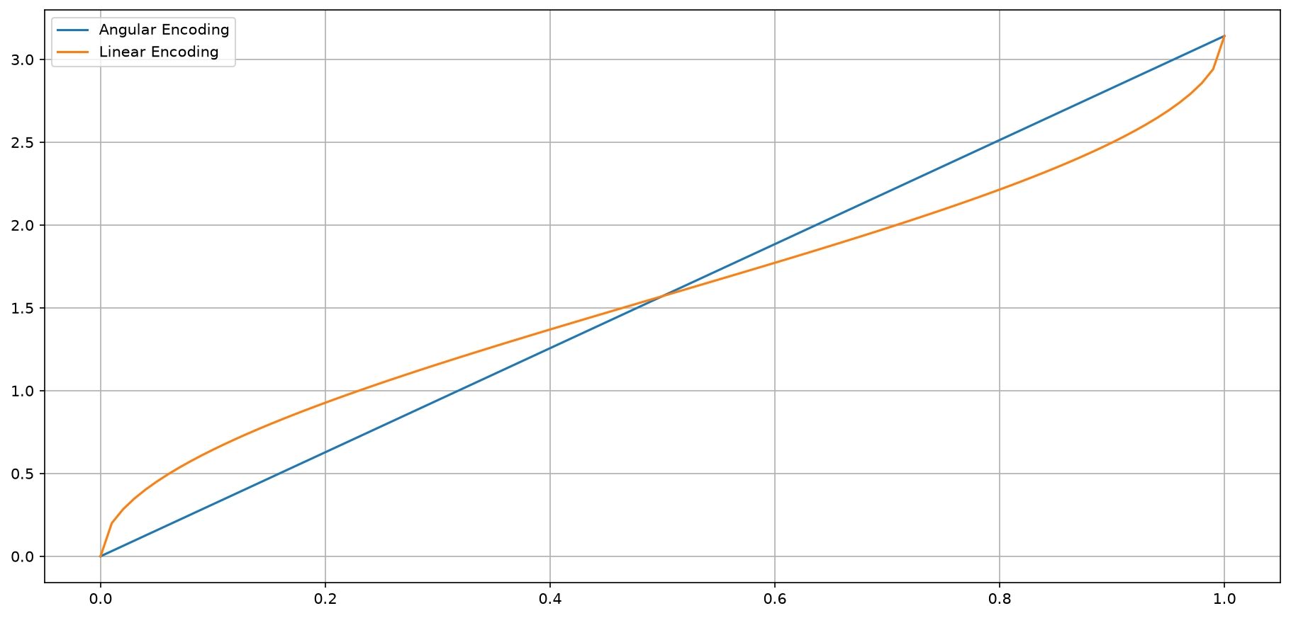
The Models operate different angle encodings:
given a scalar input \(x\), the
AngularModelencodes it with a \(\theta\) angle of
given a scalar input \(x\), the
LinearModelencodes it with a \(\theta\) angle of
import numpy as np
import matplotlib.pyplot as plt

X = [x / 100 for x in range(0, 101)]
Y_angular = [np.pi * x for x in X]
Y_linear = [np.arcsin(2 * x - 1) + np.pi / 2 for x in X]
plt.figure(figsize=(15, 7), dpi=150)
plt.plot(X, Y_angular)
plt.plot(X, Y_linear)
plt.legend(["Angular Encoding", "Linear Encoding"])
plt.grid()
plt.show()
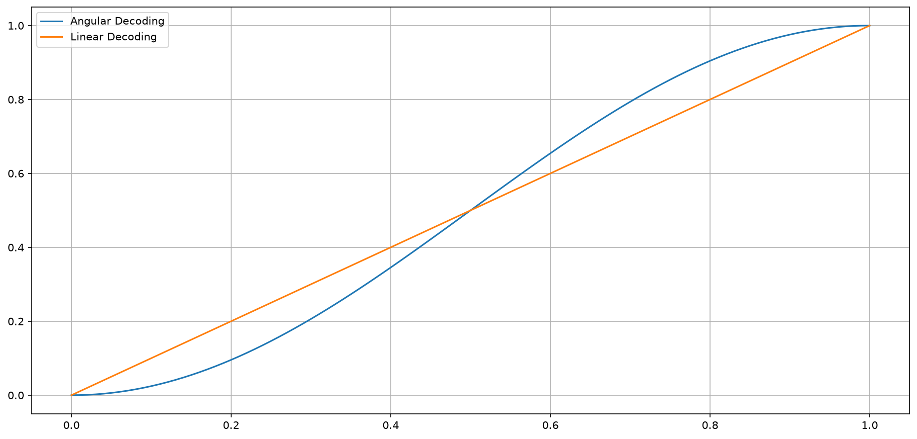
The decoding by means of the measurement probability is: $\( \text{Probability of measuring } \lvert 1 \rangle = \sin^2 \left( \frac{\theta}{2} \right)\)$
Hence, for \(\tau = 1\) the LinearModel elicitates the non-linearity by inverting it:
X = [x / 100 for x in range(0, 101)]
Y_angular = [np.square(np.sin((np.pi * x) / 2)) for x in X]
Y_linear = [np.square(np.sin((np.arcsin(2 * x - 1) + np.pi / 2) / 2)) for x in X]
plt.figure(figsize=(15, 7), dpi=150)
plt.plot(X, Y_angular)
plt.plot(X, Y_linear)
plt.legend(["Angular Decoding", "Linear Decoding"])
plt.grid()
plt.show()
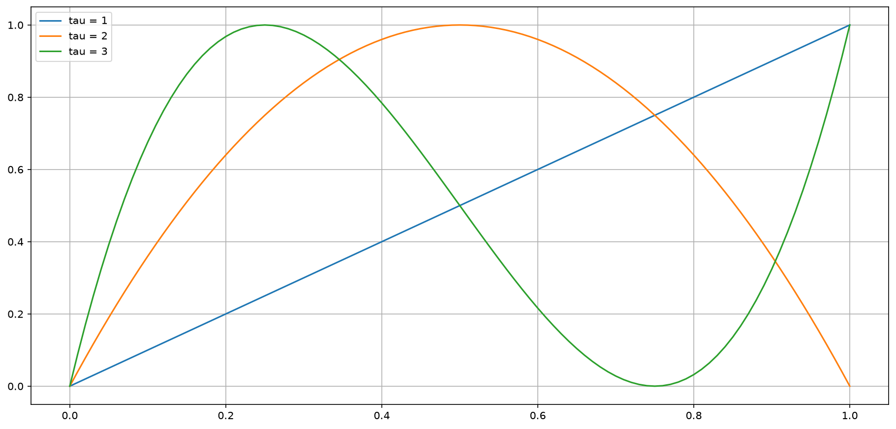
BEWARE: For \(\tau > 1\), one individual fractional rotation no longer maps its input
directly to a linear measurement probability (i.e., the LinearModel loses its linearity):
This does not mean every longer window is nonlinear in the same way. If the same value \(x\) is repeated for all \(\tau\) events, the fractional angles add back to the \(\tau=1\) angle and \(P(1)=x\). For a window containing different values, however, the accumulated inverse-sine angles generally do not encode the arithmetic mean linearly. The plots below expose that distinction.
max_tau = 3

X = [x / 100 for x in range(0, 101)]
Y = list()
for tau in range(1, max_tau + 1):
    Y.append([np.square(np.sin((np.arcsin(2 * x - 1) + np.pi / 2) / 2 * tau)) for x in X])

plt.figure(figsize=(15, 7), dpi=150)
labels = list()
for i in range(0, max_tau):
    plt.plot(X, Y[i])
    plt.grid()
    labels.append(f"tau = {i + 1}")
plt.legend(labels)
plt.show()
Input Test
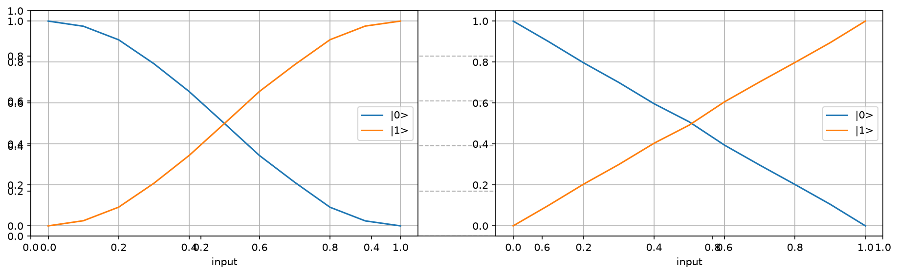
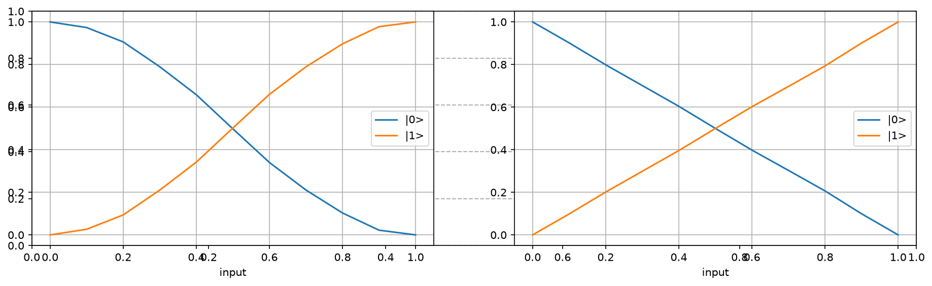
This experiment compares outcome probabilities for the Angular model (left) and Linear model (right) over inputs \(x \in [0,1]\) at fixed \(\tau\).
input_samples = 10
\(\tau\) = 1
tau = 1
import pandas as pd


def test_concat_counts(dataframe, counts, label_name, label_value, shots):
    # Store in the dataset (normalizing probabilities)
    counts[label_name] = label_value
    try:
        counts["0"] = counts["0"] / shots
    except KeyError:
        counts["0"] = 0
    try:
        counts["1"] = counts["1"] / shots
    except KeyError:
        counts["1"] = 0
    # Cast counts as dataframe to concatenate them
    counts = pd.DataFrame([counts])
    dataframe = pd.concat([dataframe, pd.DataFrame(counts)], ignore_index=True)
    return dataframe


def test_input(model, input_samples, tau=1, x_label="input"):
    dataframe = pd.DataFrame()
    shots = 10_000
    inputs = [s / input_samples for s in range(0, input_samples + 1)]
    for i in inputs:
        print(f"Input = {i}  ", end="\r")
        model.clear()
        # Encode the input and measure
        for _ in range(0, tau):
            model.encode(i, dim=0)
        counts = model.measure(shots)
        dataframe = test_concat_counts(dataframe, counts, x_label, i, shots)
    print("                        ")
    return dataframe
df_angular_input = test_input(
    AngularModel(1, tau),
    input_samples,
    tau,
    x_label="input",
)
df_angular_input
Input = 0.0
Input = 0.1
Input = 0.2
Input = 0.3
Input = 0.4
Input = 0.5
Input = 0.6
Input = 0.7
Input = 0.8
Input = 0.9
Input = 1.0
| 0 | input | 1 | |
|---|---|---|---|
| 0 | 1.0000 | 0.0 | 0.0000 |
| 1 | 0.9748 | 0.1 | 0.0252 |
| 2 | 0.9086 | 0.2 | 0.0914 |
| 3 | 0.7920 | 0.3 | 0.2080 |
| 4 | 0.6563 | 0.4 | 0.3437 |
| 5 | 0.5006 | 0.5 | 0.4994 |
| 6 | 0.3432 | 0.6 | 0.6568 |
| 7 | 0.2127 | 0.7 | 0.7873 |
| 8 | 0.0910 | 0.8 | 0.9090 |
| 9 | 0.0244 | 0.9 | 0.9756 |
| 10 | 0.0000 | 1.0 | 1.0000 |
df_linear_input = test_input(
    LinearModel(1, tau),
    input_samples,
    tau,
    x_label="input",
)
df_linear_input
Input = 0.0
Input = 0.1
Input = 0.2
Input = 0.3
Input = 0.4
Input = 0.5
Input = 0.6
Input = 0.7
Input = 0.8
Input = 0.9
Input = 1.0
| 0 | input | 1 | |
|---|---|---|---|
| 0 | 1.0000 | 0.0 | 0.0000 |
| 1 | 0.9004 | 0.1 | 0.0996 |
| 2 | 0.7962 | 0.2 | 0.2038 |
| 3 | 0.7003 | 0.3 | 0.2997 |
| 4 | 0.5965 | 0.4 | 0.4035 |
| 5 | 0.5078 | 0.5 | 0.4922 |
| 6 | 0.3943 | 0.6 | 0.6057 |
| 7 | 0.2968 | 0.7 | 0.7032 |
| 8 | 0.2022 | 0.8 | 0.7978 |
| 9 | 0.1055 | 0.9 | 0.8945 |
| 10 | 0.0000 | 1.0 | 1.0000 |
def plot_versus(dataframe1, dataframe2, x_label):
    plt.figure(figsize=(15, 4), dpi=150)
    plt.grid(linestyle="--", linewidth=1)

    plt.subplot(1, 2, 1)
    dataframe1.plot(x=x_label, y=["0", "1"], kind="line", ax=plt.gca())
    plt.legend(["|0>", "|1>"])
    plt.grid()

    plt.subplot(1, 2, 2)
    dataframe2.plot(x=x_label, y=["0", "1"], kind="line", ax=plt.gca())
    plt.legend(["|0>", "|1>"])
    plt.grid()

    plt.show()
plot_versus(
    df_angular_input,
    df_linear_input,
    x_label="input",
)
\(\tau\) = 10
tau = 10
df_angular_input = test_input(AngularModel(1, tau), input_samples, tau, x_label="input")
df_linear_input = test_input(LinearModel(1, tau), input_samples, tau, x_label="input")
Input = 0.0
Input = 0.1
Input = 0.2
Input = 0.3
Input = 0.4
Input = 0.5
Input = 0.6
Input = 0.7
Input = 0.8
Input = 0.9
Input = 1.0

Input = 0.0
Input = 0.1
Input = 0.2
Input = 0.3
Input = 0.4
Input = 0.5
Input = 0.6
Input = 0.7
Input = 0.8
Input = 0.9
Input = 1.0
plot_versus(df_angular_input, df_linear_input, x_label="input")
Queries Test
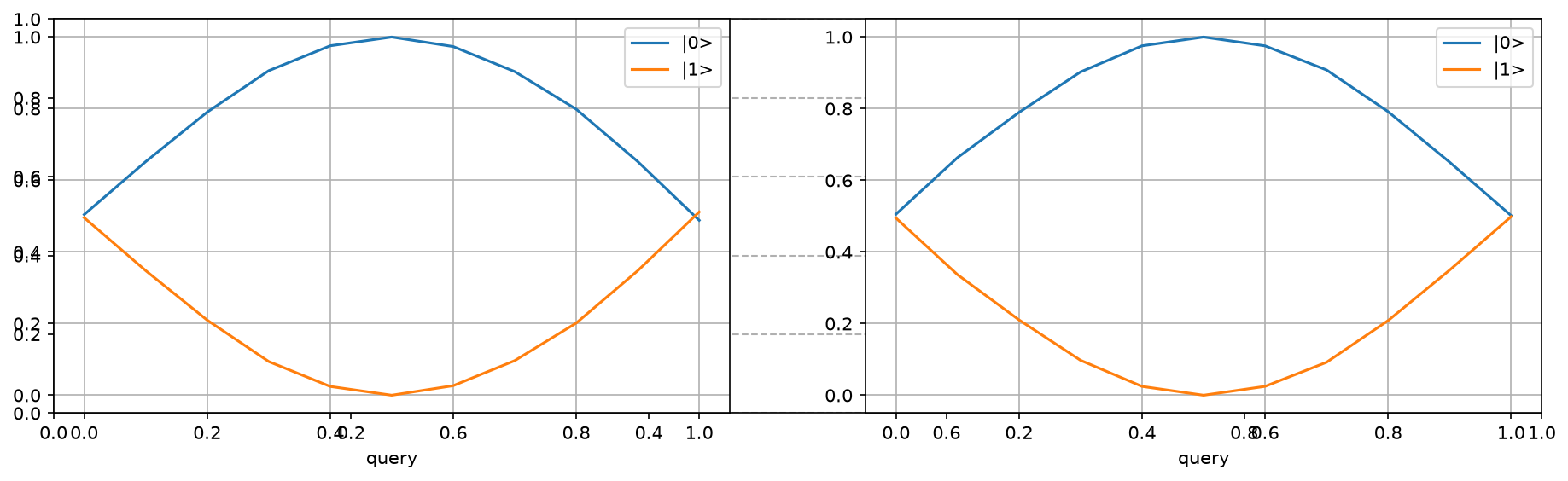
This experiment fixes \(x=0.5\) and \(\tau=1\), then compares outcome probabilities after applying query values sampled from \([0,1]\). The Angular model is shown on the left and the Linear model on the right.
query_samples = 10
def test_query(model, query_samples, x_label="query"):
    dataframe = pd.DataFrame()
    shots = 10_000
    queries = [s / query_samples for s in range(0, query_samples + 1)]
    for query in queries:
        print(f"Query = {query}  ", end="\r")
        model.clear()
        # Encode always .5 events
        model.encode(0.5, dim=0)
        # then apply the query
        model.query([query])
        # and measure
        counts = model.measure(shots)
        dataframe = test_concat_counts(dataframe, counts, x_label, query, shots)
    print("                        ")
    return dataframe
df_angular_query = test_query(AngularModel(1, 1), query_samples, x_label="query")
df_linear_query = test_query(LinearModel(1, 1), query_samples, x_label="query")
plot_versus(df_angular_query, df_linear_query, x_label="query")
Query = 0.0
Query = 0.1
Query = 0.2
Query = 0.3
Query = 0.4
Query = 0.5
Query = 0.6
Query = 0.7
Query = 0.8
Query = 0.9
Query = 1.0

Query = 0.0
Query = 0.1
Query = 0.2
Query = 0.3
Query = 0.4
Query = 0.5
Query = 0.6
Query = 0.7
Query = 0.8
Query = 0.9
Query = 1.0
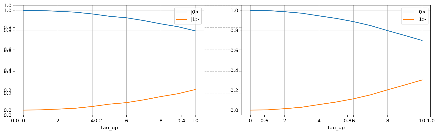
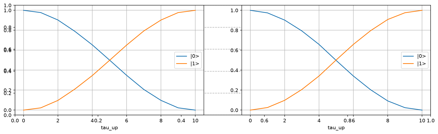
\(\tau_{\uparrow}\) Test
\(\tau_{\uparrow} \leq \tau\) is the number of events \(x=\) intensity in a sequence of \(\tau\) events (the remaining events are \(x=0\)).
For example, considering a sequence long \(\tau = 5\), with \(\tau_{\uparrow} = 3\) events of intensity \(=0.8\), a possible actual sequence could be:
tau = 10
def test_tau_up(model, intensity=1, x_label="tau_up"):
    dataframe = pd.DataFrame()
    shots = 10_000
    for tau_up in range(0, model.tau + 1):
        print(f"Tau_up = {tau_up}/{model.tau}    ", end="\r")
        model.clear()
        # Encode the tau_up events
        for _ in range(0, tau_up):
            model.encode(intensity, dim=0)
        counts = model.measure(shots)
        dataframe = test_concat_counts(dataframe, counts, x_label, tau_up, shots)
    print("                        ")
    return dataframe
df_angular_tau_up = test_tau_up(AngularModel(1, tau), intensity=1, x_label="tau_up")
df_linear_tau_up = test_tau_up(LinearModel(1, tau), intensity=1, x_label="tau_up")
plot_versus(df_angular_tau_up, df_linear_tau_up, x_label="tau_up")
Tau_up = 0/10
Tau_up = 1/10
Tau_up = 2/10
Tau_up = 3/10
Tau_up = 4/10
Tau_up = 5/10
Tau_up = 6/10
Tau_up = 7/10
Tau_up = 8/10
Tau_up = 9/10
Tau_up = 10/10

Tau_up = 0/10
Tau_up = 1/10
Tau_up = 2/10
Tau_up = 3/10
Tau_up = 4/10
Tau_up = 5/10
Tau_up = 6/10
Tau_up = 7/10
Tau_up = 8/10
Tau_up = 9/10
Tau_up = 10/10
df_angular_tau_up = test_tau_up(AngularModel(1, tau), intensity=0.7, x_label="tau_up")
df_linear_tau_up = test_tau_up(LinearModel(1, tau), intensity=0.7, x_label="tau_up")
plot_versus(df_angular_tau_up, df_linear_tau_up, x_label="tau_up")
Tau_up = 0/10
Tau_up = 1/10
Tau_up = 2/10
Tau_up = 3/10
Tau_up = 4/10
Tau_up = 5/10
Tau_up = 6/10
Tau_up = 7/10
Tau_up = 8/10
Tau_up = 9/10
Tau_up = 10/10

Tau_up = 0/10
Tau_up = 1/10
Tau_up = 2/10
Tau_up = 3/10
Tau_up = 4/10
Tau_up = 5/10
Tau_up = 6/10
Tau_up = 7/10
Tau_up = 8/10
Tau_up = 9/10
Tau_up = 10/10
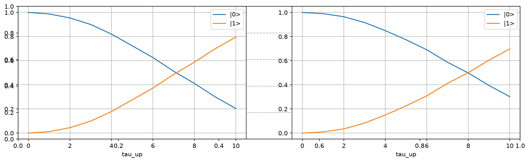
df_angular_tau_up = test_tau_up(AngularModel(1, tau), intensity=0.5, x_label="tau_up")
df_linear_tau_up = test_tau_up(LinearModel(1, tau), intensity=0.5, x_label="tau_up")
plot_versus(df_angular_tau_up, df_linear_tau_up, x_label="tau_up")
Tau_up = 0/10
Tau_up = 1/10
Tau_up = 2/10
Tau_up = 3/10
Tau_up = 4/10
Tau_up = 5/10
Tau_up = 6/10
Tau_up = 7/10
Tau_up = 8/10
Tau_up = 9/10
Tau_up = 10/10

Tau_up = 0/10
Tau_up = 1/10
Tau_up = 2/10
Tau_up = 3/10
Tau_up = 4/10
Tau_up = 5/10
Tau_up = 6/10
Tau_up = 7/10
Tau_up = 8/10
Tau_up = 9/10
Tau_up = 10/10
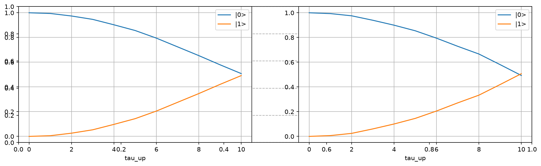
df_angular_tau_up = test_tau_up(AngularModel(1, tau), intensity=0.3, x_label="tau_up")
df_linear_tau_up = test_tau_up(LinearModel(1, tau), intensity=0.3, x_label="tau_up")
plot_versus(df_angular_tau_up, df_linear_tau_up, x_label="tau_up")
Tau_up = 0/10
Tau_up = 1/10
Tau_up = 2/10
Tau_up = 3/10
Tau_up = 4/10
Tau_up = 5/10
Tau_up = 6/10
Tau_up = 7/10
Tau_up = 8/10
Tau_up = 9/10
Tau_up = 10/10

Tau_up = 0/10
Tau_up = 1/10
Tau_up = 2/10
Tau_up = 3/10
Tau_up = 4/10
Tau_up = 5/10
Tau_up = 6/10
Tau_up = 7/10
Tau_up = 8/10
Tau_up = 9/10
Tau_up = 10/10