Introduction to quantum-robot

Research provenance

This tutorial introduces the architecture developed in Quantum-like Modeling of Cognitive Architectures for Robotics. The one-qubit model is presented and evaluated in A Preliminary Study for a Quantum-like Robot Perception Model. The multi-sensory extension is published in Multi-sensory Integration in a Quantum-Like Robot Perception Model.

Historical experiments in these papers also used IBM Quantum simulators and hardware; remote hardware execution is not part of the current package backend.

quantum-robot is a Python package for quantum-like perception modeling for robotics. Its bundled Qiskit backend builds quantum circuits and samples their statevectors locally on a classical computer.

The basic components of quantum-robot are the following:

• Models, which encode a temporal window and produce a measured state;

• bursts, which turn that state into a normalized scalar signal;

• qUnits, which run a model and burst together as an independently timed processing unit.

The following conceptual example introduces the interpretation shared by these components.

Concepts

The sleeping dead cat

A man is in his living room. He sees his cat standing still on a shelf. Nothing but some light movements of the cat’s fur is noticed by the man, who cannot decide whether the cat is dead (and the perceived movement is due to an air current) or if it is just asleep.

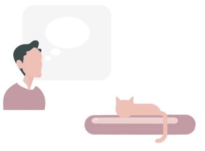
Right now he is experiencing a superposition of conscious states, because the perceptual stimuli that he receives are not strong enough to make him clearly feel that the cat is sleeping, neither that the cat is dead.

Over time, his consciousness oscillates between the two superposition states (at least, until he does not receive a stronger stimulus that makes him certain about one of the two situations)

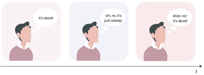
Modeling Consciousness with Quantum Mechanics

Quantum-like (QL) perception models in cognitive sciences reproduce this behavior by exploiting quantum systems properties. Considering the most simple quantum system, the qubit, QL models can represent this kind of uncertain belief state.

A qubit is a two-state quantum-mechanical system (e.g., the spin of the electron in which the two states can be taken as spin up and spin down).

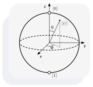
In quantum computing, a qubit is the basic unit of quantum information (the quantum version of the classical binary bit). Whether in a classical system a bit has to be in one state or the other (namely, 0 or 1), a qubit can be in a coherent superposition of both states simultaneously.

Measuring the qubit’ state causes its collapse on one of the two states, i.e., the qubit’ state pass from a superposition of states to being a single, defined state. A measurement stops the evolution of the system over time and forces its state into one of the two basis states (the ones in superposition). When the system is not observed anymore, it resumes its evolution over time.

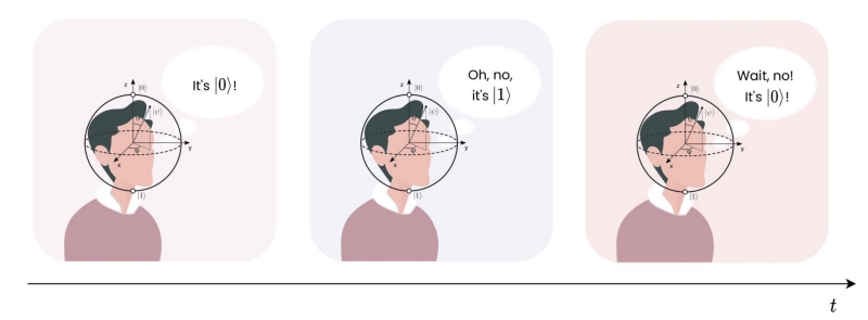
[Through the superposition] “the two alternatives exist at the perceptual-cognitive level. Then, they pass at the decisional and conscientious level towards a selection of the two subsisting alternatives. An alternative logical structure is delineated, a structure of the simultaneous YES and NO” (Elio Conte)

In this alternative logical structure, out cat is dead and yet sleeps simultaneously.

The package uses the same mathematical structure to model the robot’s belief and decision mechanism:

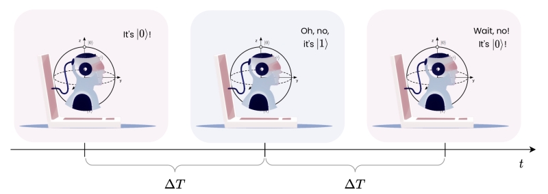
Based on the perceptual stimuli received, the robot represents its knowledge by means of a simulated quantum system. When a measure occurs, the system collapses to a defined state, which is the robot’s current measured decision state or “conscious” state. Hence, after collecting sensorial data for a specific period of time \(\Delta T\), a measurement occurs:

Implementation

The executable example below follows one signal through the two operations that later run inside a qUnit:

• The sensorial input is a normalized signal from the outside world. For example, 0/1 for “cat seems dead”/”cat seems asleep.”

• A quantum-like model accumulates that input for a temporal window \(\Delta T\) (encoding) and then measures the encoded state (decoding).

• A burst translates the decoded state into the normalized output that can be passed onward.

In a running architecture, a qUnit wraps the model and burst and repeats this sequence in its own timed process. Here we perform the same steps directly so each operation remains visible; the qUnit itself is introduced after the model demonstration.

Sensorial Input

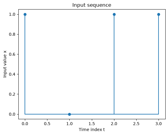
Consider a temporal window containing four binary events:

tau = 4

sequence = [
    1,  # The cat is asleep!
    0,  # The cat is dead!
    1,  # The cat is asleep!
    1,  # The cat is asleep!
]

To display the events in the considered temporal window:

import matplotlib.pyplot as plt

plt.figure()
plt.stem(sequence, linefmt="C0-", markerfmt="C0o", basefmt="C0-")
plt.xlabel("Time index t")
plt.ylabel("Input value x")
plt.title("Input sequence")
plt.show()

Model

The model accumulates binary data over a temporal window and encodes it by rotating a state vector. Measurement then produces a binary outcome sampled from the resulting quantum probability distribution.

Information encoding

A single-qubit model (\(n=1\)) encodes the binary input over a temporal window of \(\tau = 4\) samples:

from qrobot.models import AngularModel

model = AngularModel(n=1, tau=tau)

In order to understand how such model works, we can define our event sequence

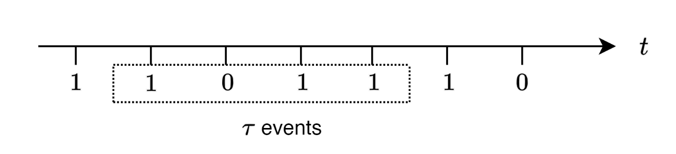
as follows:

\[ \Sigma = [1, 0, 1, 1] \]

As previously said, we associate the binary event \(\alpha_i = 0\) (“the cat is dead”) with the basis state \(\lvert 0 \rangle\) and the binary event \(\alpha_i = 1\) (“the cat is asleep”) with the basis state \(\lvert 1 \rangle\).

We define the frequency of an event associated with a basis state as:

\[ \tau_{\lvert 0 \rangle}=1 \quad\quad \tau_{\lvert 1 \rangle}=3 \]

So, the relative frequency of an event associated with a basis state is:

\[ f_{\lvert 0 \rangle}=\frac{1}{4} \quad\quad f_{\lvert 1 \rangle}=\frac{3}{4} \]

Now, we encode such information in the qubit in the Bloch sphere representation’s angle \(\theta\) of a qubit:

\[ \theta = \pi f_{\lvert 1 \rangle} \]

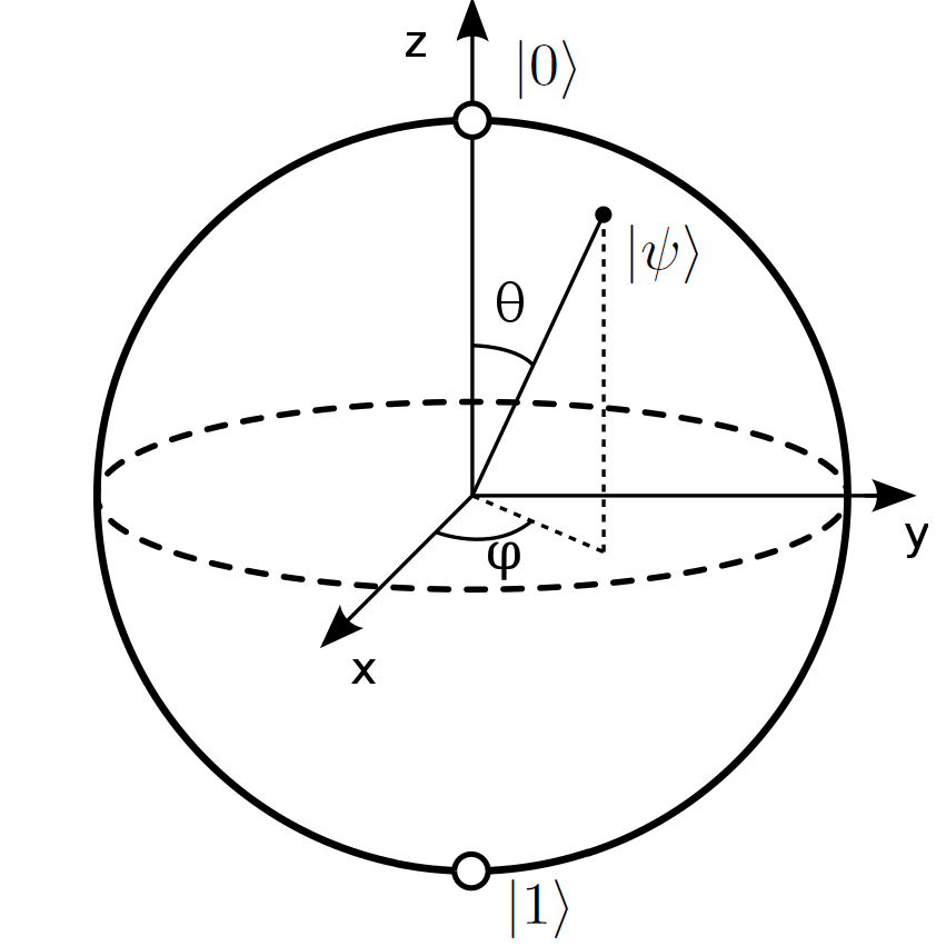
Note that we consider here the AngularModel, which encodes information directly on the angle of the Bloch sphere representation. Other models are available.

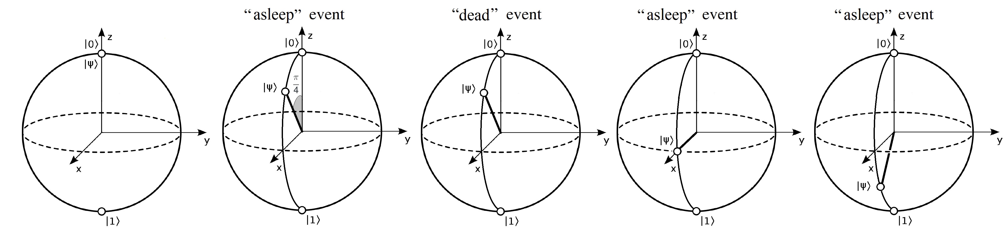
In order to encode such information, we initialize the qubit \(\lvert \psi \rangle\) at \(\lvert 0 \rangle\) and we use a unitary operator \(U\) to apply a fractional rotation of \(\pi/\tau\) along the \(y\) axis of the Bloch sphere representation. This operator has to be applied to the qubit \(\tau_{\lvert 1 \rangle}\) times for our sequence of events \(\Sigma\) (i.e., frequency of “the cat is asleep” events) in order to obtain the desired encoding of \(\theta = \pi f_{\lvert 1 \rangle}\).

To apply to a qubit a fractional rotation around the \(y\) axis of the Bloch sphere representation we need a \(R_y\) gate, which equates to a rotation around the \(y\) axis by \(\theta\) radians:

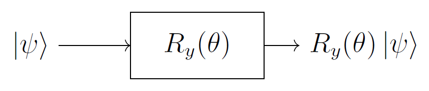
The correspondent operator is the unitary operator \(R_y\):

\[\begin{split} R_y(\theta) = \exp\left({-i\frac{\theta}{2}Y}\right) = \begin{bmatrix} \cos \frac{\theta}{2}& -\sin \frac{\theta}{2}\\ \sin \frac{\theta}{2}& \cos \frac{\theta}{2} \end{bmatrix}. \end{split}\]

We can see in our temporal window how the qubit’s state vector evolves in the Bloch sphere representation:

With the quantum-robot package, we can use the encode method of our model object to encode event data in the model:

model.clear()  # Keep this cell repeatable by discarding any earlier encoding.

for t in range(0, model.tau):  # loop throug the event sequence
    model.encode(sequence[t], dim=0)

We can see how then our model built a quantum circuit applying the rotation gates when needed:

model.print_circuit()

   ┌─────────┐┌───────┐┌─────────┐┌─────────┐
q: ┤ Ry(π/4) ├┤ Ry(0) ├┤ Ry(π/4) ├┤ Ry(π/4) ├
   └─────────┘└───────┘└─────────┘└─────────┘

From the diagram it is possible to notice how we have a rotation for every \(\lvert 1 \rangle\) event and a null rotation for every \(\lvert 0 \rangle\) event.

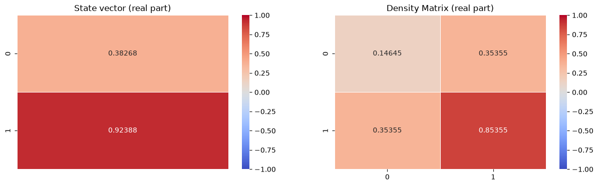
After encoding the input sequence, the model has the following state:

model.plot_state_mat()

Information decoding

The input distribution is now encoded in the model’s qubit. Decoding defines how that representation becomes an observable result.

One can use indirect techniques (Nielsen and Chuang 2010; K. M. Hangos and Ruppert 2011) or direct measurements as a decisions based on the belief state \(\lvert\psi\rangle\) (Caves et al. 2002)

In here, we consider the measurement itself as the decoding process for the model. Indeed, for a single qubit we have the following probabilities of measuring one of the two basis states:

\[ P(\lvert0\rangle) = \cos^2 \left(\frac{\theta}{2}\right) \quad\quad P(\lvert1\rangle) = \sin^2 \left(\frac{\theta}{2}\right) \]

This inherently provides a way of interpolate low-level data in a belief state (the \(\lvert\psi\rangle\) state) and then operate a decision on it. In fact, the information carried by the qubits represents a certain degree of belief (represented by the \(\theta\) encoding), and a single measurement represents a decision based on this knowledge (decision-making interpretation of the measurement).

With quantum-robot, we can easily operate the measurement on the model after having encoded our data into it:

counts = model.measure()

The measurement outcome is then:

import json

print("Measurement outcome:")
print(json.dumps(counts, sort_keys=True, indent=4))

Measurement outcome:
{
    "0": 1
}

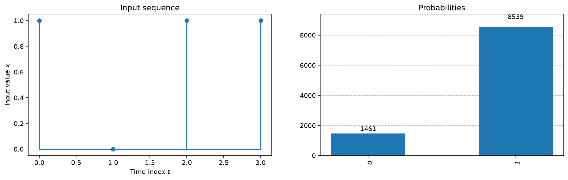
We can repeat the measurement 10,000 times to see that the outcome distribution converges to the encoded information:

counts = model.measure(shots=10_000)

print("Aggregated binary outcomes of the circuit:")
print(json.dumps(counts, sort_keys=True, indent=4))

Aggregated binary outcomes of the circuit:
{
    "0": 1461,
    "1": 8539
}

From the raw counts we can obtain the relative frequencies and compare them with the input sequence shape:

from qiskit.visualization import plot_histogram

plt.figure(figsize=(15, 4), dpi=150)

ax1 = plt.subplot(1, 2, 1)
ax1.stem(sequence, linefmt="C0-", markerfmt="C0o", basefmt="C0-")
ax1.set_xlabel("Time index t")
ax1.set_ylabel("Input value x")
ax1.set_title("Input sequence")

ax2 = plt.subplot(1, 2, 2)
plot_histogram(counts, ax=ax2)
ax2.set_ylabel("")
ax2.set_title("Probabilities")

plt.show()

Burst

The model above ends with a measured bit string. A burst is the small rule that translates such a state into the normalized scalar signal used by the rest of the architecture. For example, OneBurst returns the fraction of bits measured as 1, while ZeroBurst returns the fraction measured as 0:

from qrobot.bursts import OneBurst, ZeroBurst

measured_state = model.decode()
print("Measured state:", measured_state)
print("OneBurst output:", OneBurst()(measured_state))
print("ZeroBurst output:", ZeroBurst()(measured_state))

Measured state: 1
OneBurst output: 1.0
ZeroBurst output: 0.0

This is the bridge between the quantum-like representation and an ordinary signal: the model decides which state was measured, and the burst decides how that state should be read. In the one-dimensional cat example, either burst produces 0.0 or 1.0; with multiple dimensions it can also produce an intermediate value.

Architecture framework

qUnit

A qUnit packages the operations demonstrated above into a repeating worker: it samples input, lets its model accumulate one temporal window, applies the query and measurement, converts the measured state with its burst, and publishes the resulting scalar. Thus the model and burst are not parallel stages outside the qUnit; they are the qUnit’s internal processing mechanism.

The following creates, but does not start, a basic qUnit with the same one-dimensional model and four-sample temporal window used above:

from qrobot_qunits import QUnit

basic_qunit = QUnit(
    name="basic_perception",
    model=AngularModel(n=1, tau=tau),
    burst=OneBurst(),
    sampling_period=0.1,
)
basic_qunit

QUnit "basic_perception-88e47b"
     name:	basic_perception
     id:	basic_perception-88e47b
     model:	[model: AngularModel, n: 1, tau: 4]
     burst:	<class 'qrobot.bursts.oneburst.OneBurst'>
     query:	[0.0]
     sampling_period:	0.1

At this point the qUnit is only configured: no worker has been started and no Redis connection is needed. The qUnits tutorial gives the complete overview creating sensorial interfaces, connecting qUnits into layers, starting and stopping their workers, inspecting Redis state, and visualizing the resulting network.

From qUnits to a qBrain

A qBrain is the connected processing architecture formed when qUnits are wired between the robot’s sensor and actuator interfaces. It is not a separate quantum model. It is the whole signal network that organizes models operating at one or more temporal and cognitive levels:

• a sensorial interface publishes a normalized reading from the world;

• a perceptual qUnit integrates those readings and publishes a burst;

• a cognitive qUnit can integrate bursts from perceptual or other cognitive qUnits, potentially over a different temporal window;

• an actuator interface combines selected final bursts, applies its activation rule, and exposes a command to simulated or physical behavior.

The following diagram from Quantum-like Modeling of Cognitive Architectures for Robotics is included as a system-level illustration of these relationships. It shows the larger bug-like qBrain rather than the small cat example above: sensor interfaces \(s_i\) feed perceptual qUnits \(p_i\), their bursts feed cognitive qUnits \(c_i\), and selected outputs drive actuator interfaces \(a_i\).

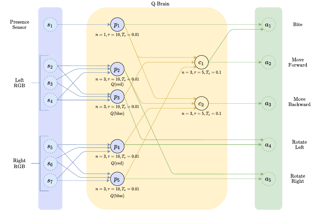
Following one arrow through that diagram gives the complete connection to the earlier sections:

• Sensor reading \(\rightarrow\) qUnit[Model Encoding \(\rightarrow\) Measurement \(\rightarrow\) Burst] \(\rightarrow\) Another qUnit or actuator interface