Bug world: a live predator/prey qBrain

Warning

qrobot_simulator is experimental. This tutorial uses scenario-specific predator/prey, sensing, movement, and rendering interfaces that may change between minor releases.

Research provenance

This tutorial implements the bug-like architecture in Quantum-like Modeling of Cognitive Architectures for Robotics. The robot, environment, and world images are archival assets of this master’s thesis work. The live two-dimensional world is generated by examples/bug_world.py using the current Redis-connected qUnit implementation.

The bug-like robot inhabits a world with blue prey and a red predator. Two RGB eyes and a frontal proximity sensor provide its evidence. Its qBrain combines that evidence into five behaviors: bite, move forward, move backward, rotate left, and rotate right.

Bug-like robot in the CoppeliaSim simulation	Predator/prey world in the CoppeliaSim simulation

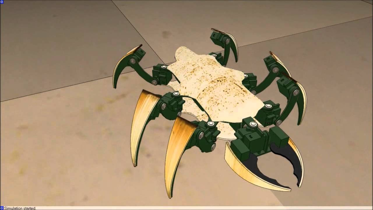
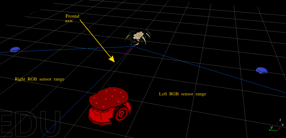
The master’s thesis evaluated the architecture in CoppeliaSim with ROS. This tutorial evaluates the same perceptual and cognitive signal graph in the packaged qrobot_simulator world.

Architecture

from IPython.display import HTML
from qrobot_qunits import RedisConfig
from qrobot_simulator.bug_world.robots.bug_robot import build_bug_qbrain
from qrobot_visualization import build_network, draw

sensors, qunits, actuators = build_bug_qbrain(RedisConfig())
architecture = draw(build_network((sensors, qunits, actuators)))
HTML(
    architecture.to_html(
        include_plotlyjs="cdn",
        full_html=False,
        config={"responsive": True},
        default_width="100%",
    )
)

Read the graph from left to right. Blue nodes are sensor interfaces and perceptual qUnits, yellow nodes are cognitive qUnits, and green nodes are actuators. Arrow colors match the layer receiving the signal. The graph is interactive, so dense wiring can be inspected with zoom and pan.

The signal path has four stages:

Sensors. bug_proximity carries frontal proximity. The bug_l* and bug_r* nodes carry the red, green, and blue channels of the left and right eyes.
Perception. Five qUnits recognize presence, left/right red, and left/right blue evidence from short sensor histories.
Cognition. bug_prey and bug_threat combine perceptual bursts over a longer temporal window into prey and danger decisions.
Actuation. Five actuator units combine those decisions into bite, forward, backward, rotate-left, and rotate-right behavior.

The two layers use different temporal windows. Perceptual units react to short sensor histories, while cognitive units integrate the resulting perceptual bursts over a longer history. Consequently, an actuator receives decisions about completed windows rather than forwarding the latest raw eye value.

Behavior	Evidence used
bite	frontal proximity and prey cognition
move forward	prey cognition and eye-feature bursts
move backward	threat cognition
rotate left	left-blue and right-red perception
rotate right	left-red and right-blue perception

Each ActuatorUnit averages its incoming bursts and publishes an activation only when that normalized value is strictly greater than its threshold. The thresholds reflect the discrete burst levels: forward combines prey cognition with the eye-feature bursts to maintain a search drive when no target is visible, backward requires a stronger threat decision, and the two-input rotation actuators require strong lateral evidence. Backward also has a larger physical gain than forward, so simultaneous opposing qBrain activations still produce retreat rather than cancelling each other.

Simulated world

BugWorld.demo() constructs the same arena and animals used by the public example. A plain actuator-driven bug body is used here:

from pprint import pprint
from qrobot_simulator.bug_world import BugWorld

world = BugWorld.demo()

pprint(world.board, sort_dicts=False)

Chessboard(columns=18, rows=12, cell_size=1.0)

pprint(world.bug, sort_dicts=False)

BugRobot(name='qBrain bug',
         x=5.5,
         y=4.0,
         heading=0.0,
         color='#704214',
         radius=0.3,
         max_speed=1.0,
         max_turn=0.7)

pprint(world.prey, sort_dicts=False)

[BluePrey(name='prey 1',
          x=9.5,
          y=6.2,
          heading=3.141592653589793,
          color='#2878d0',
          radius=0.3,
          max_speed=1.0,
          max_turn=2.0,
          motion_mode='deterministic'),
 BluePrey(name='prey 2',
          x=8.8,
          y=1.6,
          heading=2.6,
          color='#2878d0',
          radius=0.3,
          max_speed=1.0,
          max_turn=2.0,
          motion_mode='random')]

pprint(world.predator, sort_dicts=False)

RedPredator(name='predator',
            x=1.5,
            y=6.5,
            heading=-0.5,
            color='#d43c32',
            radius=0.3,
            max_speed=1.0,
            max_turn=2.0,
            motion_mode='deterministic',
            bite_period=3.0)

The world computes the exact seven normalized values consumed by the packaged sensor units:

pprint(world.readings, sort_dicts=False)

{'proximity': 0.0,
 'lr': 0.0,
 'lg': 0.0,
 'lb': 0.983198095219912,
 'rr': 0.0,
 'rg': 0.0,
 'rb': 1.0}

Each RGB eye points \(30^\circ\) away from the bug’s heading. Its response decreases with angular error and distance. Blue prey stimulate the blue eye channels, the red predator stimulates the red channels, and the frontal proximity sensor becomes active within its configured \(1.25\)-unit range and \(\pm25^\circ\) field of view. Bite contact is calculated separately from the two body radii and the configured bite reach. The simulation deliberately contains no green animal, so both green channels stay at zero.

One prey follows a repeatable curved path and the other wanders randomly; both flee nearby hunters. The predator pursues the qBrain bug. BugWorld.step() advances those animals, applies the bug’s actuator values, detects bites, respawns captured prey, and refreshes the sensor readings.

Live demo

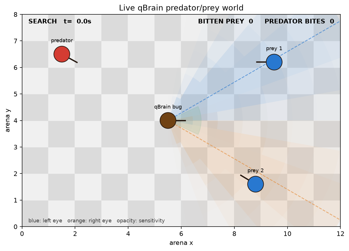
Live chessboard with qBrain bug, two blue prey, red predator, and sensor rays

The live view shows the chessboard, four robots, frontal proximity region, both RGB eye fields, current behavior, proximity region, and scores. BITTEN PREY counts successful bug bites. PREDATOR BITES counts predator contacts, with a cooldown so continuous contact is not scored once per frame.

World geometry produces sensor values; qUnits integrate those values and publish bursts; actuators select behavior; and that behavior changes the next world state. The renderer only displays this state and never infers behavior.

The red and blue perceptual units use ZeroBurst to query their target colors, while the cognitive units use OneBurst. Every readout is a one-shot measurement, so paths and firing patterns can vary even from similar geometry.

Run the example

Start Redis on localhost:6379, then run:

python examples/bug_world.py

The simulation runs until its window closes or Ctrl-C is pressed. The world refresh rate can be changed independently of the qUnit worker periods:

python examples/bug_world.py --fps 5

For a bounded or headless run:

python examples/bug_world.py --duration 20
python examples/bug_world.py --duration 10 --no-show \
  --save-world bug_live_world.png

On shutdown it stops its workers and removes only the Redis keys owned by its BugRobot.

Reference

D. Lanza, Quantum-like Modeling of Cognitive Architectures for Robotics, Zenodo, 2020.