Getting started with qUnits

Research provenance

The Redis-connected qUnit/qBrain architecture is described in Quantum-like Modeling of Cognitive Architectures for Robotics. This tutorial demonstrates the current package runtime.

Important

This tutorial starts qUnit worker processes and therefore requires a Redis server listening on localhost:6379. Install the qunits extra and start Redis before executing this page. Redis is the shared communication and observable-state sidecar for independently scheduled qUnit processes and the dashboard.

from qrobot.bursts import OneBurst, ZeroBurst
from qrobot.logger import LoggingConfig, configure_logging
from qrobot.models import AngularModel
from qrobot_qunits import QUnit, SensorialUnit
from qrobot_qunits.redis import flush_redis, redis_status
from qrobot_visualization import build_network, draw
from IPython.display import HTML
from pathlib import Path
import time

# This is application-owned logging. The library does not configure handlers
# unless this opt-in helper is called.
logging_config = LoggingConfig(
    level=10,  # logging.DEBUG
    file_path=Path(".qrobot_logs/qrobot-qunits-debug.log"),
    console=False,  # keep executed-documentation output readable
)
configure_logging(logging_config)

<Logger qrobot (DEBUG)>

Set up a basic qBrain

First, define a sensorial input:

# Layer 0 - Unit 0
l0_unit0 = SensorialUnit("l0_unit0", sampling_period=0.1, logging_config=logging_config)

Then, choose a model and the desired bursts:

print(AngularModel(n=2, tau=10))
print(ZeroBurst())
print(OneBurst())

[model: AngularModel, n: 2, tau: 10]
<qrobot.bursts.zeroburst.ZeroBurst object at 0x77ea5c3692b0>
<qrobot.bursts.oneburst.OneBurst object at 0x77ea5c3692b0>

You can use objects like those to create a basic qBrain:

# Layer 1 - Unit 0
l1_unit0 = QUnit(
    name="l1_unit0",
    model=AngularModel(n=1, tau=10),
    burst=OneBurst(),
    sampling_period=0.1,
    in_qunits={0: l0_unit0.id},  # Will receive Input from l0_unit0, dim 0
    logging_config=logging_config,
)

# Layer 1 - Unit 1
l1_unit1 = QUnit(
    name="l1_unit1",
    model=AngularModel(n=1, tau=25),
    burst=ZeroBurst(),
    sampling_period=0.1,
    in_qunits={0: l0_unit0.id},  # Will receive input from l0_unit0, dim 0
    logging_config=logging_config,
)

Modify l1_unit1’s query, then inspect the complete architecture:

l1_unit1.query = [0.8]

Show code cell source

Hide code cell source

architecture = draw(build_network(([l0_unit0], [l1_unit0, l1_unit1], [])))
HTML(
    architecture.to_html(
        include_plotlyjs="cdn",
        full_html=False,
        config={"responsive": True},
        default_width="100%",
    )
)

Read the graph from left to right. The blue sensorial unit publishes one scalar reading to both perceptual qUnits. Each arrow identifies that input dependency. The two qUnits use different temporal windows and bursts, which are summarized directly in their node labels; l1_unit1 also shows the query set above. You can zoom or pan the graph to inspect the labels.

Check the default input for l0_unit0:

l0_unit0.scalar_reading

0.0

Real-time processing

Both qUnits sample every 0.1 seconds, but they integrate different numbers of samples. l1_unit0 decides every \(10\times0.1=1\) second; l1_unit1 decides every \(25\times0.1=2.5\) seconds.

The important direction of time is:

1. during a window, the qUnit reads and encodes incoming samples;

2. at the right edge, it applies its query to the accumulated state;

3. it performs one binary measurement and publishes the corresponding burst;

4. it resets the model and starts accumulating the next window, while the previous burst remains visible.

Therefore, an output drawn just after time \(t\) describes the completed window immediately before \(t\). It is not a decision about the current sensor sample.

The next cell runs the system in real time, records a snapshot every refresh_time, and changes l0_unit0.scalar_reading once per second:

import time
import json
from random import randint
from IPython.display import clear_output

statuses = []
refresh_time = 0.25  # Plot four Redis snapshots per second.
input_change_period = 1.0
run_duration = 30
units = (l0_unit0, l1_unit0, l1_unit1)

for unit in units:
    unit.start()

try:
    for i in range(int(run_duration / refresh_time)):
        time.sleep(refresh_time)
        clear_output(wait=True)

        # Keep each random reading for one second, so both qUnits integrate
        # visible blocks of evidence rather than unrelated high-rate noise.
        if i % int(input_change_period / refresh_time) == 0:
            l0_unit0.scalar_reading = randint(0, 1000) / 1000

        status = redis_status()
        statuses.append(status)
        print(json.dumps(status, indent=1, sort_keys=True))
        print(round((i + 1) * refresh_time, 2), f"/{run_duration} seconds")

    latest_bursts = {
        l1_unit0.name: l1_unit0.get_burst_output(),
        l1_unit1.name: l1_unit1.get_burst_output(),
    }
finally:
    for unit in reversed(units):
        unit.stop()

{
 "l0_unit0-746c90 class": "SensorialUnit",
 "l0_unit0-746c90 output": "0.418",
 "l1_unit0-2e0f5f class": "QUnit",
 "l1_unit0-2e0f5f in_qunits": "{\"0\": \"l0_unit0-746c90\"}",
 "l1_unit0-2e0f5f output": "1.0",
 "l1_unit0-2e0f5f query": "[0.0]",
 "l1_unit0-2e0f5f state": "1",
 "l1_unit1-fd1b4f class": "QUnit",
 "l1_unit1-fd1b4f in_qunits": "{\"0\": \"l0_unit0-746c90\"}",
 "l1_unit1-fd1b4f output": "1.0",
 "l1_unit1-fd1b4f query": "[0.8]",
 "l1_unit1-fd1b4f state": "0"
}
30.0 /30 seconds

These are the latest outputs that were captured before stopping the units:

latest_bursts

{'l1_unit0': 1.0, 'l1_unit1': 1.0}

stop() already removes the keys owned by each unit:

redis_status()

{}

To flush the redis to clean all traces (should not be necessary if the qUnits processing loops stopped correctly):

flush_redis()
redis_status()

{}

Visualize the results

The recorded values show how signals evolve over that interval:

Show code cell source

Hide code cell source

import numpy as np
import pandas as pd
import matplotlib.pyplot as plt

status_df = pd.DataFrame(statuses)
units = [l0_unit0.id + " output", l1_unit0.id + " output", l1_unit1.id + " output"]
status_df = status_df[units]
status_df = status_df.astype(np.float64)
status_df.index = (status_df.index + 1) * refresh_time

sensor_key = l0_unit0.id + " output"
fast_key = l1_unit0.id + " output"
slow_key = l1_unit1.id + " output"


def plot_unit_decisions(unit_specs):
    """Plot sensor evidence followed by one row per qUnit decision stream."""
    fig, axes = plt.subplots(
        1 + len(unit_specs),
        1,
        figsize=(15, 2.7 * (1 + len(unit_specs))),
        sharex=True,
    )
    axes = np.atleast_1d(axes)
    sensor_axis = axes[0]
    sensor_axis.step(status_df.index, status_df[sensor_key], where="post", color="green")
    sensor_axis.set_title("Sensor readings and query targets")

    for decision_axis, (unit, burst_key, burst_label, color) in zip(
        axes[1:], unit_specs, strict=True
    ):
        query = unit.query[0]
        sensor_axis.axhline(query, color=color, ls="--", label=f"{unit.name} query = {query}")
        decision_axis.step(status_df.index, status_df[burst_key], where="post", color=color)
        decision_axis.set_title(burst_label)

        first_decision = status_df[burst_key].dropna().index[0]
        window_duration = unit.model.tau * unit.sampling_period
        decision_times = np.arange(first_decision, run_duration + refresh_time, window_duration)
        decision_axis.vlines(
            decision_times,
            ymin=0,
            ymax=1,
            colors="gray",
            linestyles="dotted",
            linewidth=1,
        )
        # With one qUnit, align its boundaries across evidence and output.
        if len(unit_specs) == 1:
            sensor_axis.vlines(
                decision_times,
                ymin=0,
                ymax=1,
                colors="gray",
                linestyles="dotted",
                linewidth=1,
            )

    sensor_axis.legend(loc="upper right")
    for axis in axes:
        axis.set_ylim(-0.05, 1.05)
        axis.set_ylabel("Value")
    axes[-1].set_xlabel("Elapsed time (s)")
    fig.tight_layout()
    plt.show()


fast_plot = (
    l1_unit0,
    fast_key,
    "Fast qUnit decision (previous 1-second window)",
    "goldenrod",
)
slow_plot = (
    l1_unit1,
    slow_key,
    "Slow qUnit decision (previous 2.5-second window)",
    "blue",
)

plot_unit_decisions([fast_plot, slow_plot])

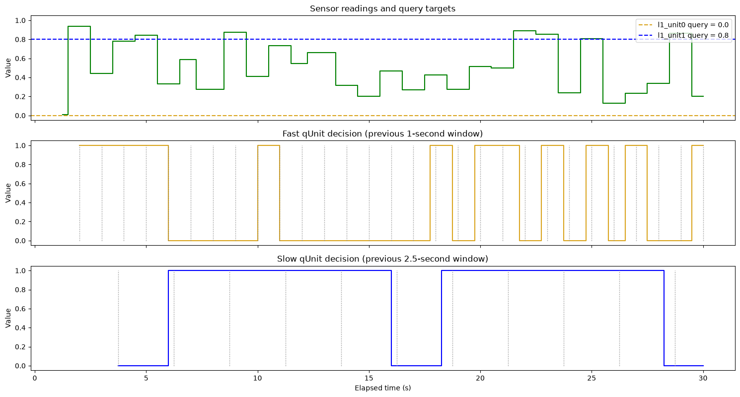
The top row contains only evidence and targets: the green trace is the sensor input, and the dashed lines are the two queries. The middle and bottom rows are the binary decision streams coming from each qUnit.

Each qUnit turns the previous temporal window of input values into one query-relative, probabilistic decision.

For the “fast” unit l1_unit0:

• due to OneBurst it publishes 0 when the measured is state \(\lvert 0 \rangle\)

• due to the query 0.0, the \(\lvert 0 \rangle\) state is more likely to be measured the closest the input is to 0.0

For the “swow” unit l1_unitq:

• due to ZeroBurst it publishes 1 when the measured is state \(\lvert 0 \rangle\)

• due to the query 0.8, the \(\lvert 0 \rangle\) state is more likely to be measured the closest the input is to 0.8

Focusing on l1_unit0:

print(l1_unit0)
plot_unit_decisions([fast_plot])

QUnit "l1_unit0-2e0f5f"
     name:	l1_unit0
     id:	l1_unit0-2e0f5f
     model:	[model: AngularModel, n: 1, tau: 10]
     burst:	<class 'qrobot.bursts.oneburst.OneBurst'>
     query:	[0.0]
     sampling_period:	0.1

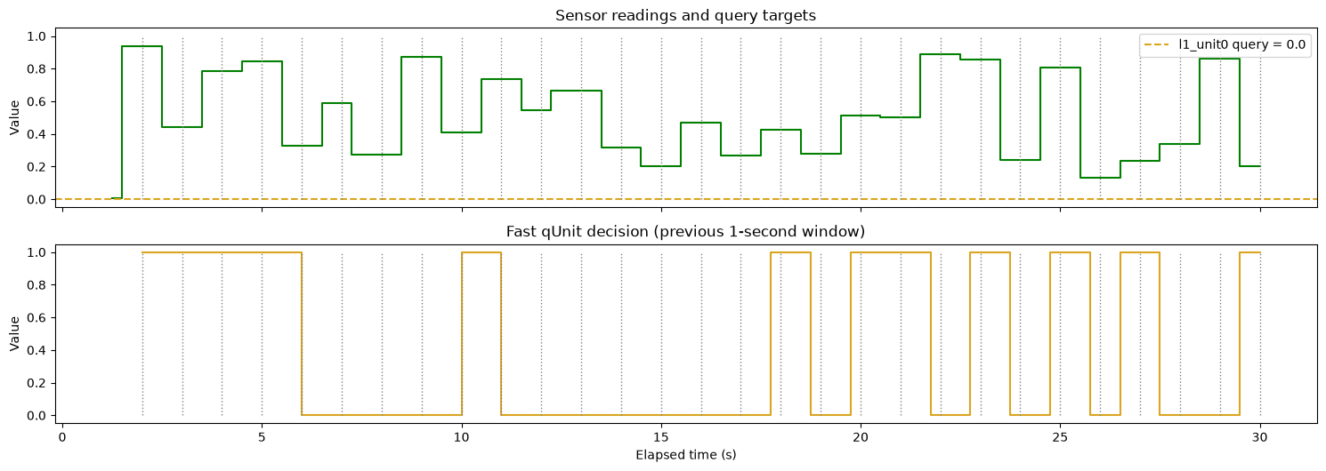
With query 0.0, l1_unit0 tends to emit 0 for windows near 0.0 and 1 for windows farther from 0.0. Each output comes from a finite quantum measurement, so repeated runs can differ even when their inputs match.

Focusing on l1_unit1:

print(l1_unit1)
plot_unit_decisions([slow_plot])

QUnit "l1_unit1-fd1b4f"
     name:	l1_unit1
     id:	l1_unit1-fd1b4f
     model:	[model: AngularModel, n: 1, tau: 25]
     burst:	<class 'qrobot.bursts.zeroburst.ZeroBurst'>
     query:	[0.8]
     sampling_period:	0.1

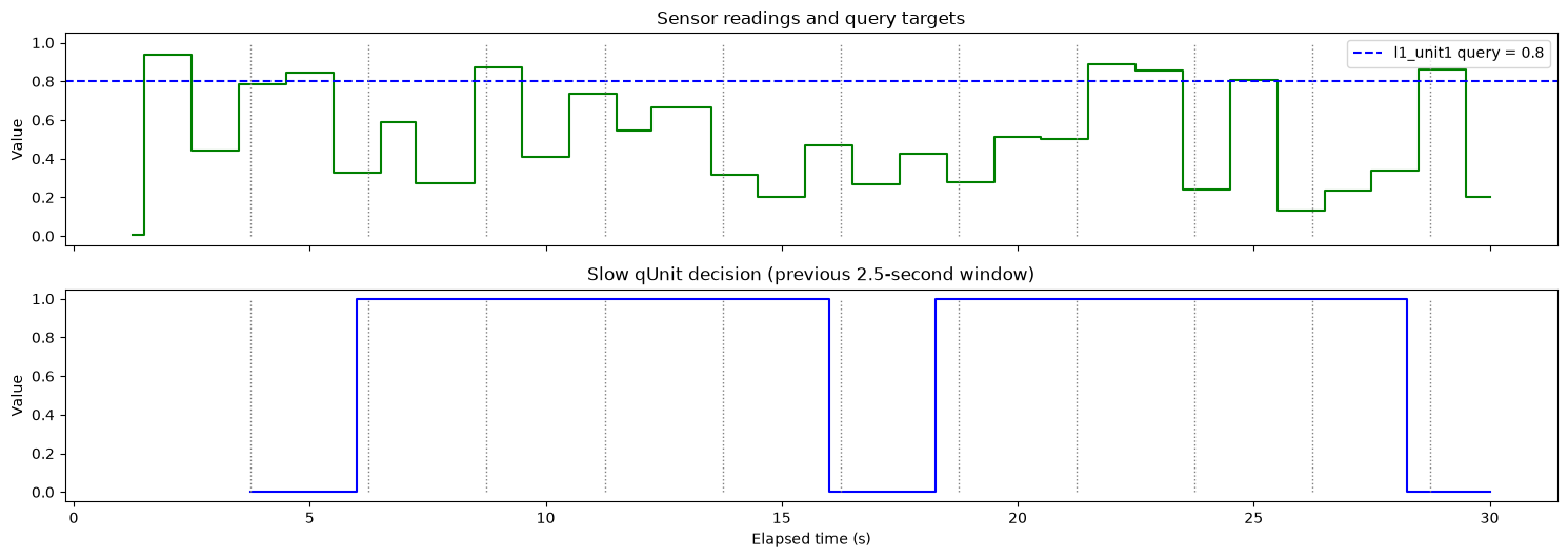
With query 0.8, the zero-bit ZeroBurst tends to emit 1 for windows near 0.8 and 0 for more distant windows. Finite measurement makes individual outputs stochastic rather than a reproducible arithmetic summary such as a mean.

Logging and debugging qUnits

Logging is opt-in. Configure a rotating-free debug file and the console in the application that creates qUnits:

# The same config is passed to each unit above. This is important on platforms
# using `spawn`, where workers do not inherit the parent process's handlers.
logging_config

LoggingConfig(level=10, file_path=PosixPath('.qrobot_logs/qrobot-qunits-debug.log'), console=False)

The resulting log can be inspected without relying on a library-managed file:

print("\n".join(logging_config.file_path.read_text().splitlines()[-20:]))

2026-09-02 21:33:12,288 — qrobot.l0_unit0-746c90 — DEBUG — Writing input on redis
2026-09-02 21:33:12,290 — qrobot.l1_unit1-fd1b4f — DEBUG — Temporal window event 7/25
2026-09-02 21:33:12,292 — qrobot.l1_unit1-fd1b4f — DEBUG — input_vector=[0.418]
2026-09-02 21:33:12,304 — qrobot.l1_unit0-2e0f5f — DEBUG — Temporal window event 3/10
2026-09-02 21:33:12,306 — qrobot.l1_unit0-2e0f5f — DEBUG — input_vector=[0.418]
2026-09-02 21:33:12,391 — qrobot.l0_unit0-746c90 — DEBUG — scalar_reading=0.418
2026-09-02 21:33:12,391 — qrobot.l0_unit0-746c90 — DEBUG — Writing input on redis
2026-09-02 21:33:12,393 — qrobot.l1_unit1-fd1b4f — DEBUG — Temporal window event 8/25
2026-09-02 21:33:12,396 — qrobot.l1_unit1-fd1b4f — DEBUG — input_vector=[0.418]
2026-09-02 21:33:12,407 — qrobot.l1_unit0-2e0f5f — DEBUG — Temporal window event 4/10
2026-09-02 21:33:12,410 — qrobot.l1_unit0-2e0f5f — DEBUG — input_vector=[0.418]
2026-09-02 21:33:12,479 — qrobot.l1_unit1-fd1b4f — INFO — Stopping QUnit
2026-09-02 21:33:12,487 — qrobot.l1_unit1-fd1b4f — INFO — Cleaning redis
2026-09-02 21:33:12,492 — qrobot.l1_unit0-2e0f5f — INFO — Stopping QUnit
2026-09-02 21:33:12,494 — qrobot.l0_unit0-746c90 — DEBUG — scalar_reading=0.418
2026-09-02 21:33:12,495 — qrobot.l0_unit0-746c90 — DEBUG — Writing input on redis
2026-09-02 21:33:12,503 — qrobot.l1_unit0-2e0f5f — INFO — Cleaning redis
2026-09-02 21:33:12,507 — qrobot.l0_unit0-746c90 — INFO — Stopping SensorialUnit
2026-09-02 21:33:12,514 — qrobot.l0_unit0-746c90 — INFO — Cleaning redis
2026-09-02 21:33:12,541 — qrobot.redis — INFO — Flushing Redis database

print(
    "Time window time:",
    l1_unit1.sampling_period * l1_unit1.model.tau,
    "seconds",
)
matching_lines = [
    line
    for line in logging_config.file_path.read_text().splitlines()
    if "l1_unit1" in line and "Output state =" in line
]
print("\n".join(matching_lines[-10:]))

Time window time: 2.5 seconds
2026-09-02 21:32:48,053 — qrobot.l1_unit1-fd1b4f — DEBUG — Output state = 1
2026-09-02 21:32:50,672 — qrobot.l1_unit1-fd1b4f — DEBUG — Output state = 0
2026-09-02 21:32:53,289 — qrobot.l1_unit1-fd1b4f — DEBUG — Output state = 1
2026-09-02 21:32:55,907 — qrobot.l1_unit1-fd1b4f — DEBUG — Output state = 1
2026-09-02 21:32:58,520 — qrobot.l1_unit1-fd1b4f — DEBUG — Output state = 0
2026-09-02 21:33:01,127 — qrobot.l1_unit1-fd1b4f — DEBUG — Output state = 0
2026-09-02 21:33:03,727 — qrobot.l1_unit1-fd1b4f — DEBUG — Output state = 0
2026-09-02 21:33:06,339 — qrobot.l1_unit1-fd1b4f — DEBUG — Output state = 0
2026-09-02 21:33:08,956 — qrobot.l1_unit1-fd1b4f — DEBUG — Output state = 0
2026-09-02 21:33:11,564 — qrobot.l1_unit1-fd1b4f — DEBUG — Output state = 0