Monodimensional Angular Model
Research provenance
The model introduced here is presented in A Preliminary Study for a Quantum-like Robot Perception Model (2020), and later incorporated into Quantum-like Modeling of Cognitive Architectures for Robotics.
import numpy as np
import matplotlib.pyplot as plt
from qiskit.visualization import plot_histogram
from qrobot.models import AngularModel
In this notebook we present a 1-dimensional (\(n=1\)) demo for the
AngularModel class. The model integrates a sequence of normalized sensor
events in one qubit and produces a binary outcome when that qubit is measured.
n = 1
Here, we considered a time window of \(\tau > 1\).
tau = 30
For each event \(x_t\in[0,1]\), the model applies a fractional rotation \(R_y(\pi x_t/\tau)\). Since every rotation uses the same axis, the final angle is
where \(\bar{x}\) is the mean input in the temporal window. Consequently, \(P(0)=\cos^2(\theta/2)\) and \(P(1)=\sin^2(\theta/2)\).
Input definition
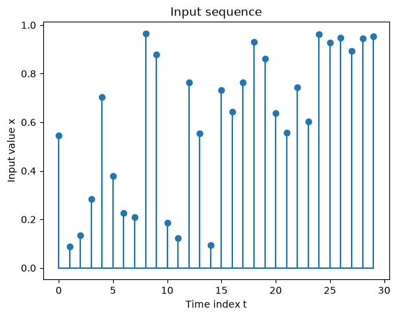
We start by defining an arbitrary continuous input sequence. Its first half spans the full normalized interval, while the second half is biased toward larger readings:
sequence = list()

# Balanced events (between 0 and 1)
for i in range(0, int(tau / 2)):
    sequence.append(np.random.randint(0, 1000) / 1000)

# Unbalanced events (balanced between .5 and 1)
for i in range(int(tau / 2), tau):
    sequence.append(np.random.randint(500, 1000) / 1000)

plt.figure()
plt.stem(sequence, linefmt="C0-", markerfmt="C0o", basefmt="C0-")
plt.xlabel("Time index t")
plt.ylabel("Input value x")
plt.title("Input sequence")
plt.show()
Encode the input in the model
We initialize the model by instantiating an object with \(n\) and \(\tau\)
model = AngularModel(n, tau)
Using the encode method, we can encode each event’s data in the model (for multidimensional inputs, a second loop is needed in order to loop through the \(n\) dimensions of the input).
model.clear()  # Keep this cell repeatable by discarding any earlier encoding.

for t in range(0, model.tau):  # loop throug the event sequence
    model.encode(sequence[t], dim=0)
The model is implemented by a Qiskit quantum circuit:
model.print_circuit()
   ┌──────────────┐┌───────────────┐┌──────────────┐┌──────────────┐»
q: ┤ Ry(0.056968) ├┤ Ry(0.0091106) ├┤ Ry(0.013928) ├┤ Ry(0.029845) ├»
   └──────────────┘└───────────────┘└──────────────┘└──────────────┘»
«   ┌──────────────┐┌──────────────┐┌──────────────┐┌──────────────┐»
«q: ┤ Ry(0.073723) ├┤ Ry(0.039584) ├┤ Ry(0.023667) ├┤ Ry(0.021991) ├»
«   └──────────────┘└──────────────┘└──────────────┘└──────────────┘»
«   ┌─────────────┐┌──────────────┐┌──────────────┐┌──────────────┐»
«q: ┤ Ry(0.10116) ├┤ Ry(0.092049) ├┤ Ry(0.019583) ├┤ Ry(0.012776) ├»
«   └─────────────┘└──────────────┘└──────────────┘└──────────────┘»
«   ┌──────────────┐┌─────────────┐┌───────────────┐┌─────────────┐»
«q: ┤ Ry(0.080111) ├┤ Ry(0.05791) ├┤ Ry(0.0099484) ├┤ Ry(0.07676) ├»
«   └──────────────┘└─────────────┘└───────────────┘└─────────────┘»
«   ┌─────────────┐┌──────────────┐┌──────────────┐┌──────────────┐»
«q: ┤ Ry(0.06744) ├┤ Ry(0.079901) ├┤ Ry(0.097599) ├┤ Ry(0.090164) ├»
«   └─────────────┘└──────────────┘└──────────────┘└──────────────┘»
«   ┌──────────────┐┌──────────────┐┌──────────────┐┌──────────────┐»
«q: ┤ Ry(0.066602) ├┤ Ry(0.058434) ├┤ Ry(0.077807) ├┤ Ry(0.063041) ├»
«   └──────────────┘└──────────────┘└──────────────┘└──────────────┘»
«   ┌─────────────┐┌──────────────┐┌──────────────┐┌─────────────┐»
«q: ┤ Ry(0.10064) ├┤ Ry(0.097075) ├┤ Ry(0.099274) ├┤ Ry(0.09341) ├»
«   └─────────────┘└──────────────┘└──────────────┘└─────────────┘»
«   ┌──────────────┐┌─────────────┐
«q: ┤ Ry(0.099065) ├┤ Ry(0.10001) ├
«   └──────────────┘└─────────────┘
Given the input we defined above, the model is in the following state:
model.plot_state_mat()
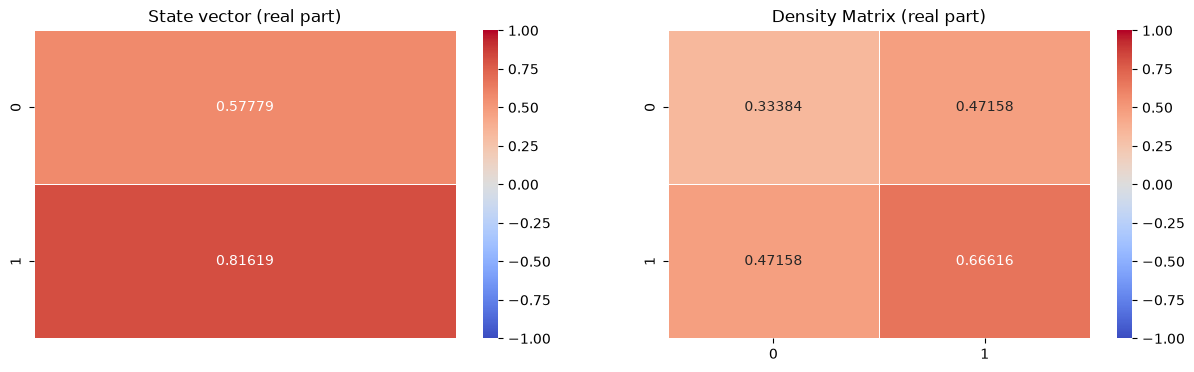
Density matrix (see Wikipedia): for a finite-dimensional state space, the most general density operator is of the form
where the coefficients \(p_{j}\) are non-negative and add up to one, and \(|\psi _{j}\rangle \langle \psi _{j}|\) is an outer product written in bra-ket notation. This represents a mixed state, with probability \( p_{j}\) that the system is in the pure state \(|\psi _{j}\rangle \).
Measurement simulation
A single call to model.decode() performs one measurement and can be
interpreted as one stochastic decision:
print(f"One-shot decision: |{model.decode()}⟩")
One-shot decision: |1⟩
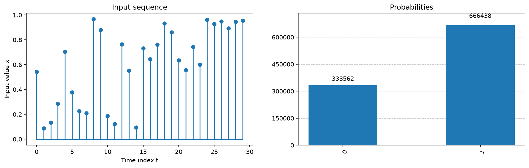
Now we instead simulate many shots to expose the probability distribution
for the two possible basis-state outcomes \(\lvert 0 \rangle\) and \(\lvert 1 \rangle\)
and validate the information encoded by the temporal window:
shots = 1000000
counts = model.measure(shots)
Raw counts for each possible outcome:
import json

print("Aggregated binary outcomes of the circuit:")
print(json.dumps(counts, sort_keys=True, indent=4))
Aggregated binary outcomes of the circuit:
{
    "0": 333562,
    "1": 666438
}
From the raw counts we can obtain the relative frequencies (aka the probabilities) and compare them with the input sequence shape:
plt.figure(figsize=(15, 4), dpi=150)

ax1 = plt.subplot(1, 2, 1)
ax1.stem(sequence, linefmt="C0-", markerfmt="C0o", basefmt="C0-")
ax1.set_xlabel("Time index t")
ax1.set_ylabel("Input value x")
ax1.set_title("Input sequence")

ax2 = plt.subplot(1, 2, 2)
plot_histogram(counts, ax=ax2)
ax2.set_ylabel("")
ax2.set_title("Probabilities")

plt.show()
References
D. Lanza, P. Solinas, and F. Mastrogiovanni, A Preliminary Study for a Quantum-like Robot Perception Model, arXiv:2006.02771, 2020.
D. Lanza, Quantum-like Modeling of Cognitive Architectures for Robotics, Zenodo, 2020.